Tutorial Page

Optimization

Below is a minimal working example that performs a topology optimization. This will run a compliance minimization with OC method.

Optimizer Configuration, and Run

import sktopt

cfg = sktopt.core.optimizers.OC_Config(
    dst_path="./result/tutorial_box_oc",
    vol_frac=sktopt.tools.SchedulerConfig.constant(
        target_value=0.4
    ),
    max_iters=10,
    record_times=10,
    export_img=True
)
optimizer = sktopt.core.OC_Optimizer(cfg, mytask)
optimizer.parameterize()
optimizer.optimize()

But before running the optimization, we need to set up the task configuration and the design variables.

Task Definition

Shape modeling and its basis function

In this example, we use skfem.ElementHex1(), which represents a first-order (linear) hexahedral element. Scikit-Topt currently supports:

• 3D: Hexahedral P1 (ElementHex1)

• 3D Tetrahedral P1 (ElementTetP1)

import skfem
import sktopt

x_len = 8.0
y_len = 8.0
z_len = 1.0
mesh_size = 0.2

mesh = sktopt.mesh.toy_problem.create_box_hex(
    x_len, y_len, z_len, mesh_size
)
e = skfem.ElementVector(skfem.ElementHex1())
basis = skfem.Basis(mesh, e, intorder=1)

Load Basis from Model File

Scikit-Topt loads meshes via scikit-fem, which internally relies on meshio. Therefore, the library supports all mesh formats that meshio supports:

Gmsh v2 (ASCII / binary)

Gmsh v4 (ASCII / binary)

When using .msh files, users may provide physical groups (surfaces/volumes) which scikit-topt interprets as boundary and subdomain tags.

import skfem
import sktopt

mesh_path = "./data/model.msh"
basis = sktopt.mesh.loader.basis_from_file(mesh_path, intorder=1)

Task Configuration

dirichlet_in_range = sktopt.mesh.utils.get_points_in_range(
    (0.0, 0.05), (0.0, y_len), (0.0, z_len)
)
dirichlet_dir = "all"

eps = mesh_size
force_in_range_0 = sktopt.mesh.utils.get_points_in_range(
    (x_len, x_len), (y_len-eps, y_len), (0, z_len)
)
force_in_range_1 = sktopt.mesh.utils.get_points_in_range(
    (x_len, x_len), (0, eps), (0, z_len)
)
force_dir_type = ["u^2", "u^2"]
force_value = [-100, 100]

boundaries = {
    "dirichlet": dirichlet_in_range,
    "force_0": force_in_range_0,
    "force_1": force_in_range_1
}
mesh = mesh.with_boundaries(boundaries)
subdomains = {"design": np.array(range(mesh.nelements))}
mesh = mesh.with_subdomains(subdomains)

e = skfem.ElementVector(skfem.ElementHex1())
basis = skfem.Basis(mesh, e, intorder=2)
E0 = 210e3
mytask = task.LinearElasticity.from_mesh_tags(
    basis,
    "all",
    force_dir_type,
    force_value,
    E0,
    0.30,
)

Results and Visualization

The results of the optimization are stored in the directory specified by cfg.dst_path. They include visualizations of the density distribution and graphs showing the evolution of optimization quantities such as compliance, volume fraction, and sensitivities.

## Examples

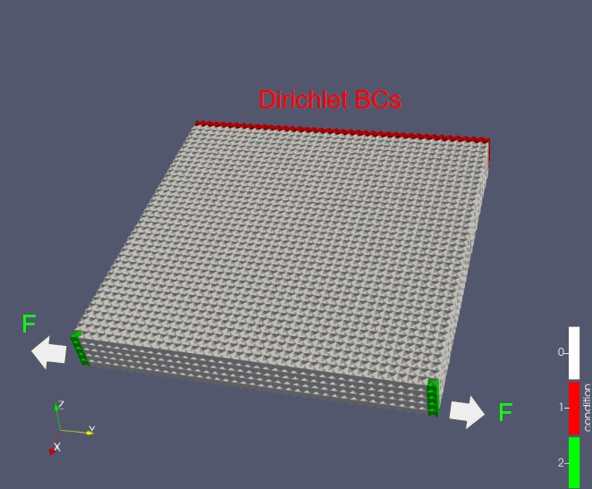
Multi-load condition visualization.

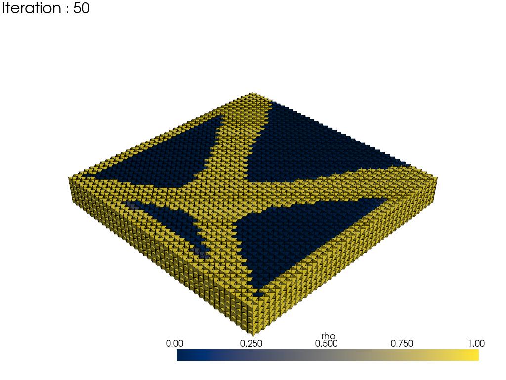
Density distribution after optimization under multi-load conditions.